Graphical User Interface Guide
The GUI starting program is defined in ErwinJr.py, which includes two
tabs: the quantum tab and the optical tab.
The quantum tab is mostly a GUI wrapper of QCLayers with a plotting canvas,
while the optical tab is for OptStrata
Quantum Tab
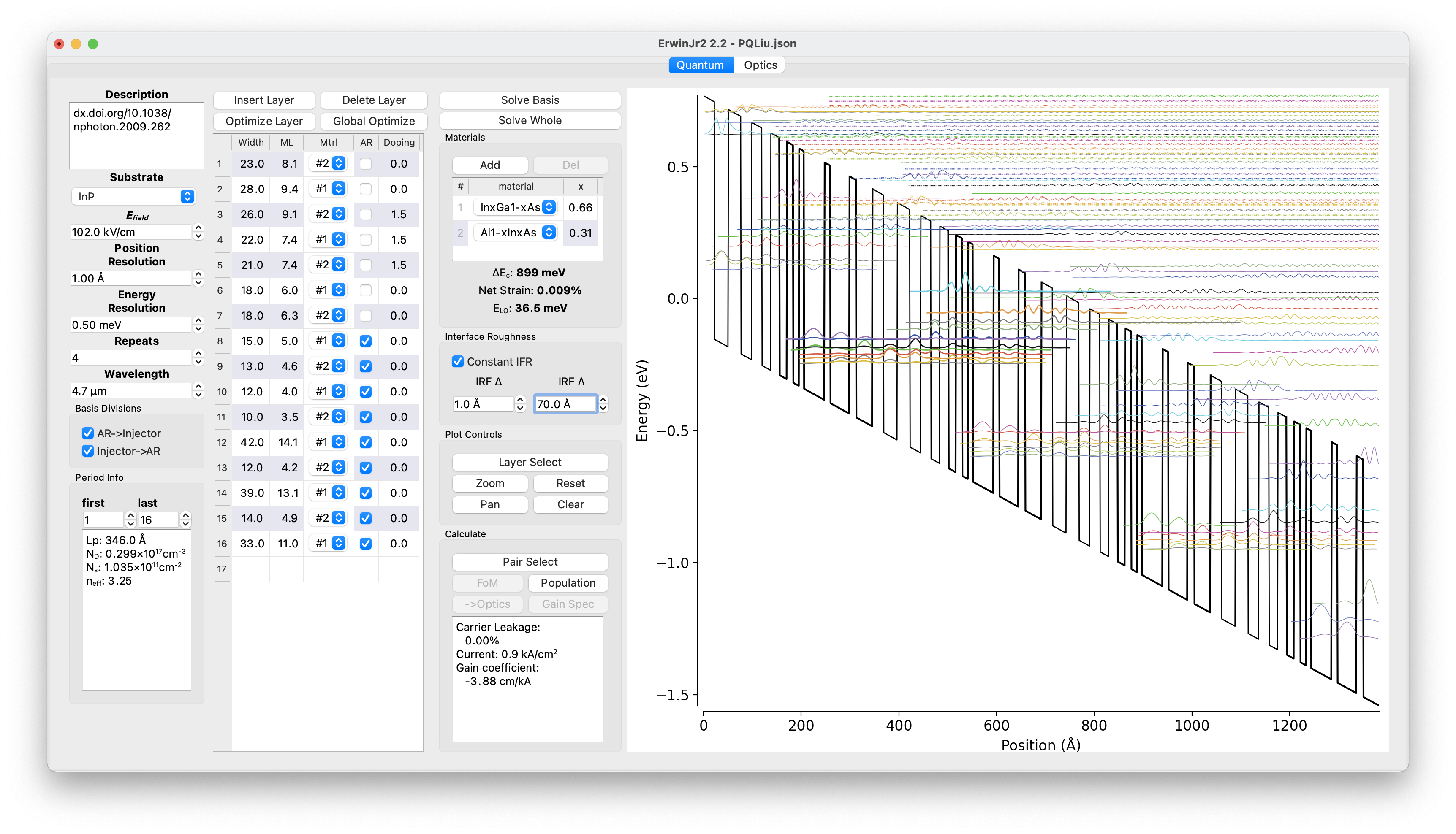
A screenshot of the ErwinJr.py quantum tab.
The interface includes 4 columns:
settingBox |
|
|---|---|
Description |
Used as a comment, not for calculation |
Substrate |
Decide substrate, can influence strain and material set |
E-field |
Global electrical field |
Position resolution |
Finite-element grid size |
Energy resolution |
Scan size for the eigen-solver root finder.
It only shows when the ODE solver is selected.
This should be smaller than the smallest energy
difference.
If this is too small it’s possible to lose some states
|
No of States Per Period |
Determines the number of states to solve for.
It only shows when the matrix solver is selected.
This should be large enough to cover the range of
interest
|
Repeats |
Number of the whole structure |
Wavelength |
The wavelength is used for optimization and for calculating global gain |
Basis Divisions |
Defined for basis solver.
See |
Period info |
Calculate the total length and doping density |
layerBox |
|
|---|---|
Layer Buttons |
Insert above a layer or delete the selected layer |
Optimize Buttons |
Start optimizing.
|
Layer Table |
Show the table that defines the layer structure |
solveBox |
|
|---|---|
Solve basis button |
Call |
Solve whole button |
Call |
Material Table |
Define the material used in the structure |
Interface Roughness |
The interface roughness \(\Delta\) and \(\Lambda\)
See
|
Plot control |
|
Calculation box |
|
The plot canvas
The black lines (or blue line if a well is selected) are the conduction band
bottom of the potential.
The states are the colored curve but thick black if selected.
Other symmetry points in the band and the plot
style of the wavefunctions can be changed from View in the menu bar.
States that are thick in line are the selected set of a single period of states.
This selected set is used to calculate the electron population distribution.
States that are dashed lines are considered not well-bounded.
Export of the figure and data, save and load actions are embedded into File menu;
temperature setting and advanced table settings are in Edit menu;
options to choose what is included in the plot are listed in View menu.
Optics Tab
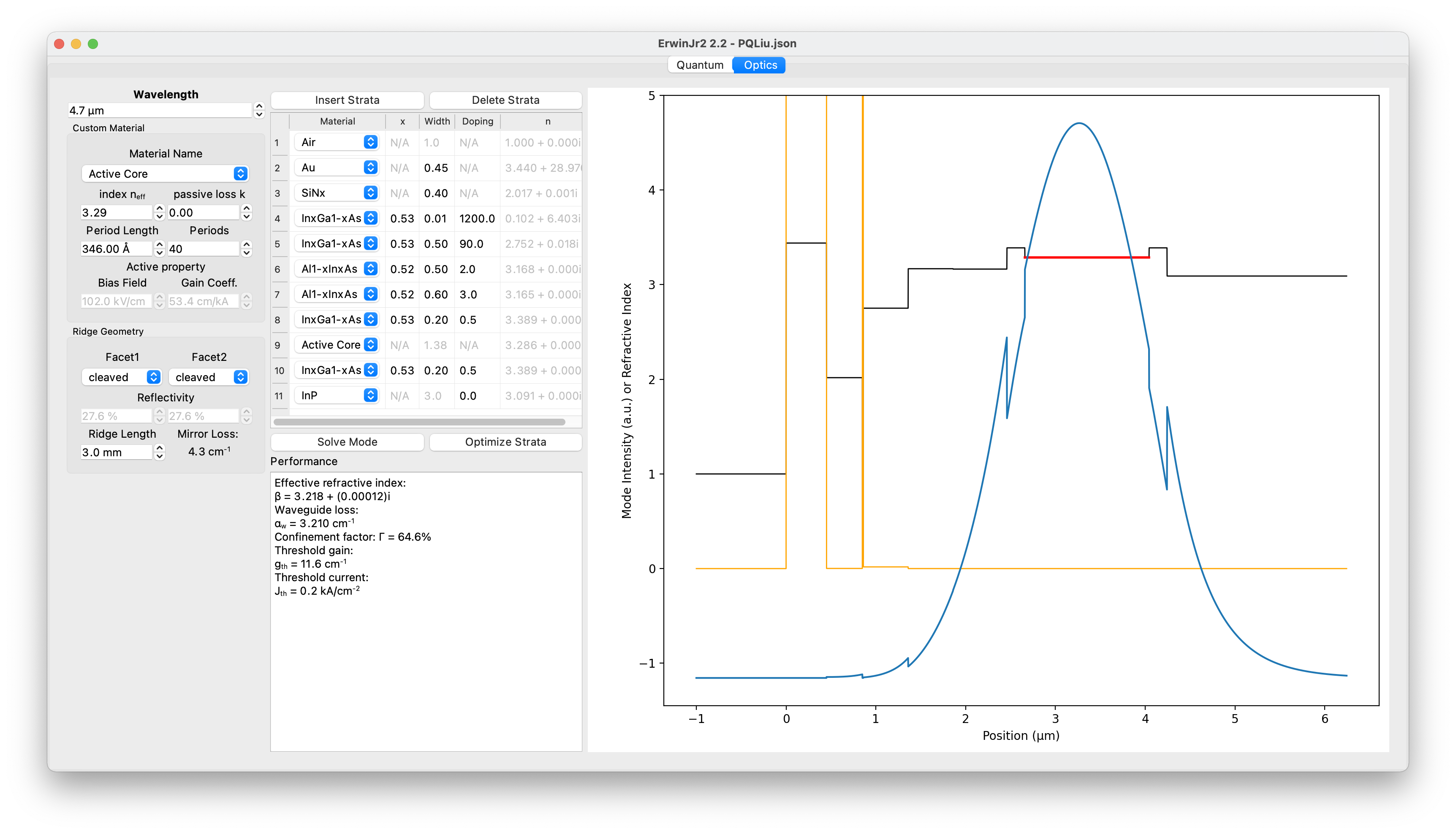
A screenshot of the ErwinJr.py quantum tab.
The interface includes 3 columns:
settingBox |
|
|---|---|
Wavelength |
Can be transferred from quantum tab but not necessarily the same |
Material Block |
Defines the customized material. For pure GUI users, it defines Active Core transferred from quantum tab
|
Ridge Geometry |
Defines the ridge facet loss for threshold gain calculation
|
strataBox |
|
|---|---|
The Strata Table |
Defines the waveguide structure.
|
Solving Block |
Solve for the first bounded mode and show its character
The optimizing is performed for the lowest threshold,
restricted to the total width of selected layers in the
pop-up window.
|
The plot canvas
The black line and orange lines are the real and imaginary parts of the refractive index, respectively. The active core can be red based on the selection in View menu.