Command Line Guide
This chapter is used as examples on how to use the code as a Python module rather than as GUI software. However, users are very encouraged to read QCLayers module and OptStrata module on how to use this package.
QC layers
The basic routine of solving a QCL structure is:
Load the structure either from a saved file or defined manually
Transform the structure to a spatial grid by
QCLayers.populate_x()Solve the structure eigenstates by
QCLayers.solve_whole()Optional the periodicity of the structure can be recognized by
QCLayers.period_recognize()With the above periodicity constructed,
QCLayers.full_population()can solve for the electron distribution
For starters we recommend to create the QCL structure in the GUI and load the structure by command line. The easiest example would be:
from ErwinJr2 import SaveLoad
from ErwinJr2.QCPlotter import plotPotential, plotWF
from ErwinJr2.QCLayers import QCLayers, auto_gain
import matplotlib.pyplot as plt
import numpy as np

qcl = QCLayers(
   substrate='InP',
   EField=51.0,
   layerWidths=[
      34.0, 14.0, 33.0, 13.0, 32.0, 15.0, 31.0, 19.0, 29.0, 23.0, 27.0, 25.0,
      27.0, 44.0, 18.0, 9.0, 57.0, 11.0, 54.0, 12.0, 45.0, 25.0],
   layerMtrls=[
      0, 1, 0, 1, 0, 1, 0, 1, 0, 1, 0, 1, 0, 1, 0, 1, 0, 1, 0, 1, 0, 1],
   layerDopings=[
      0.0, 0.0, 0.0, 0.0, 0.0, 0.0, 2.0, 2.0, 2.0, 2.0, 0.0, 0.0, 0.0, 0.0,
      0.0, 0.0, 0.0, 0.0, 0.0, 0.0, 0.0, 0.0],
   layerARs=[
      False, False, False, False, False, False, False, False, False, False,
      False, False, False, True, True, True, True, True, True, True, True,
      False],
   mtrlIFRDelta=[1.2, 1.2],
   mtrlIFRLambda=[90.0, 90.0]
)
# IFR must be manually enabled, otherwise the IFR parameters will be ignored
qcl.includeIFR = True
# or load from file
# with open("../../ErwinJr2/example/std8um.json", 'r') as f:
#     qcl = SaveLoad.qclLoad(f)

# To use customized IFR settings
# qcl.customIFR = True
# array to define individual IFR for interfaces.. the length should be the
# same as the number of layers, which means IFR parameters between layer[n]
# and layer[n+1]
# qcl.ifrDelta = [...]
# qcl.ifrLambda = [...]

qcl.populate_x()
qcl.solve_whole()
qcl.period_recognize()
qcl.full_population()
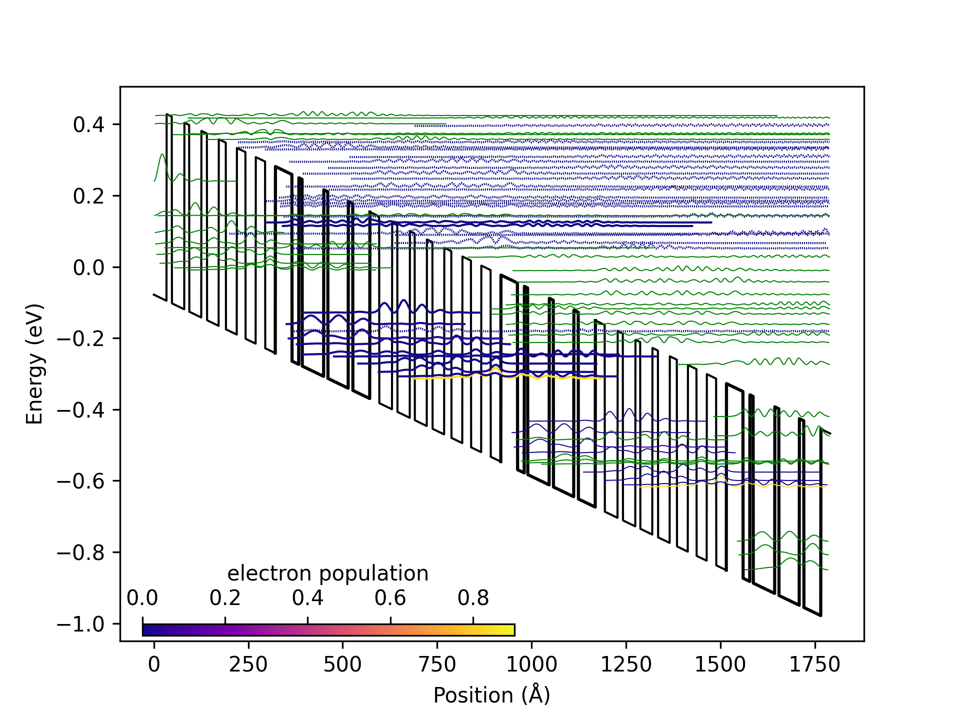
plotPotential(qcl)
plotWF(qcl)
plt.xlabel('Position (Å)')
plt.ylabel('Energy (eV)')
plt.show()
(Source code, png)

where running QCLayers.populate_x(), QCLayers.solve_whole(),
QCLayers.period_recognize(), and QCLayers.full_population()
can be replaced for short by auto_gain().
See QCLayers module for more detail.
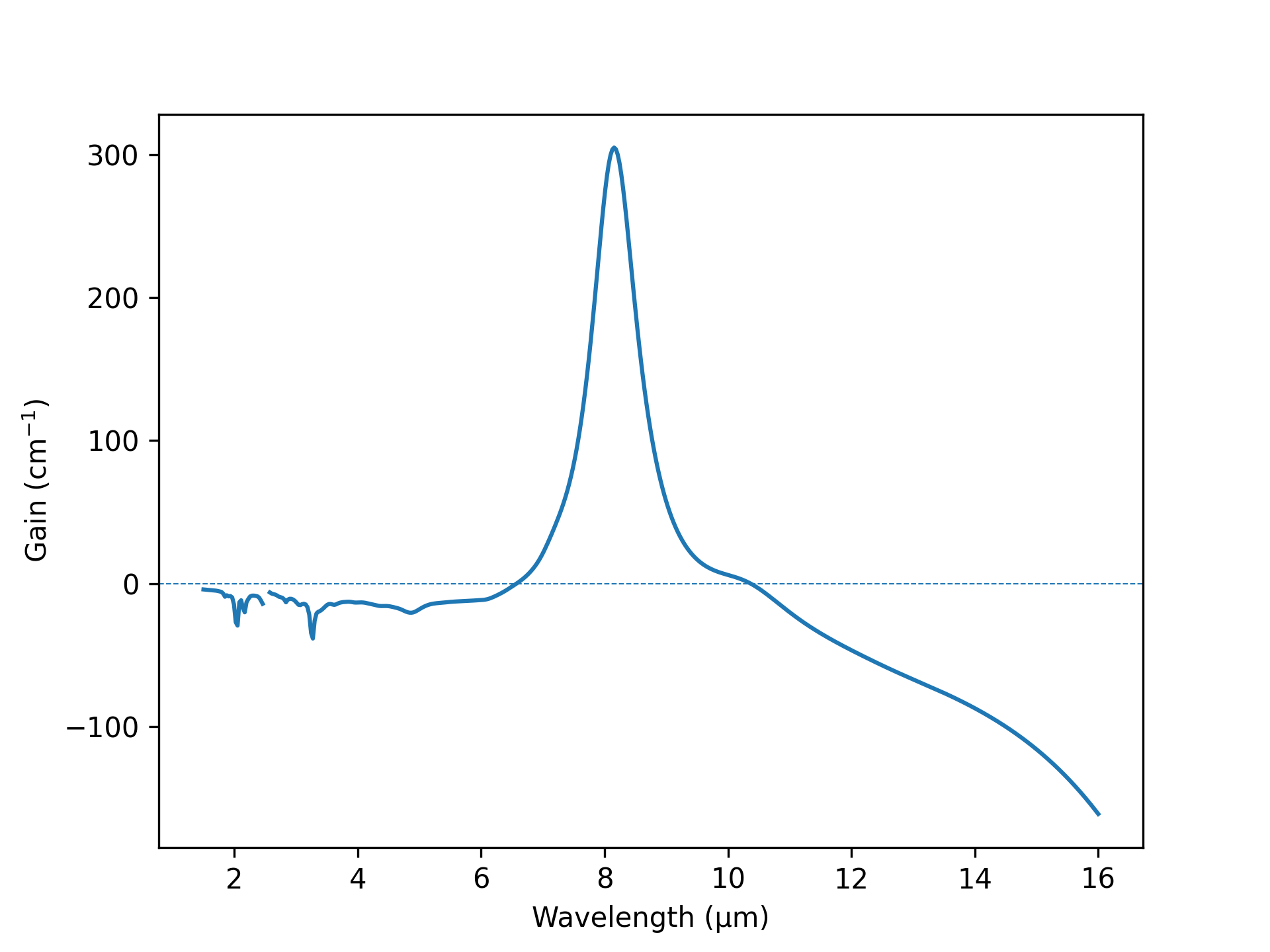
Further more, plot the gain spectrum:
wls = np.linspace(1.5, 16, 500)
plt.plot(wls, qcl.full_gain_spectrum(wls))
plt.axhline(0, ls='--', lw=0.5)
plt.xlabel('Wavelength (μm)')
plt.ylabel('Gain (cm$^{-1}$)')
plt.show()
(Source code, png)

Waveguide
Similarly the ErwinJr2.OptStrata module can also be used independent
of the GUI. See OptStrata module for more detail.
from ErwinJr2 import SaveLoad
from ErwinJr2.OptStrata import OptStrata
import numpy as np
import matplotlib
import matplotlib.pyplot as plt

strata = OptStrata(
   wl=8.0,
   materials=[
      "Air", "InP", "InP", "InP", "InP", "InxGa1-xAs", "Active Core",
      "InxGa1-xAs", "InP", "InP"],
   moleFracs=[0.0, 0.0, 0.0, 0.0, 0.0, 0.53, 0.53, 0.53, 0.53, 0.0],
   dopings=[0.0, 1000.0, 80.0, 2.0, 1.0, 0.5, 0, 0.5, 0, 0.0],
   Ls=[1.0, 0.01, 0.35, 0.5, 2.5, 0.5, 2.0895, 0.5, 5.0, 1.0],
   # the properties for the active core
   cstmIndx={"Active Core": 3.28+0j},
   cstmPrd={"Active Core": [597.0, 35]},
   cstmGain={"Active Core": 39.6}
)
# or load from file
# with open("../../ErwinJr2/example/std8um.json", 'r') as f:
#    strata = SaveLoad.optLoad(f)

beta = strata.boundModeTM()
The waveguide modeling is different from the QC layer modeling in that it is
solve analytically, meaning no discretization is made when solving for the
guided mode. However, spatial grid is needed when doing the confinement factor
integral and when plotting. the OptStrata is designed in the way that
it does not store any intermediate calculation, except for material properties,
so the spatial grid needs to be provided in any method call. So after getting
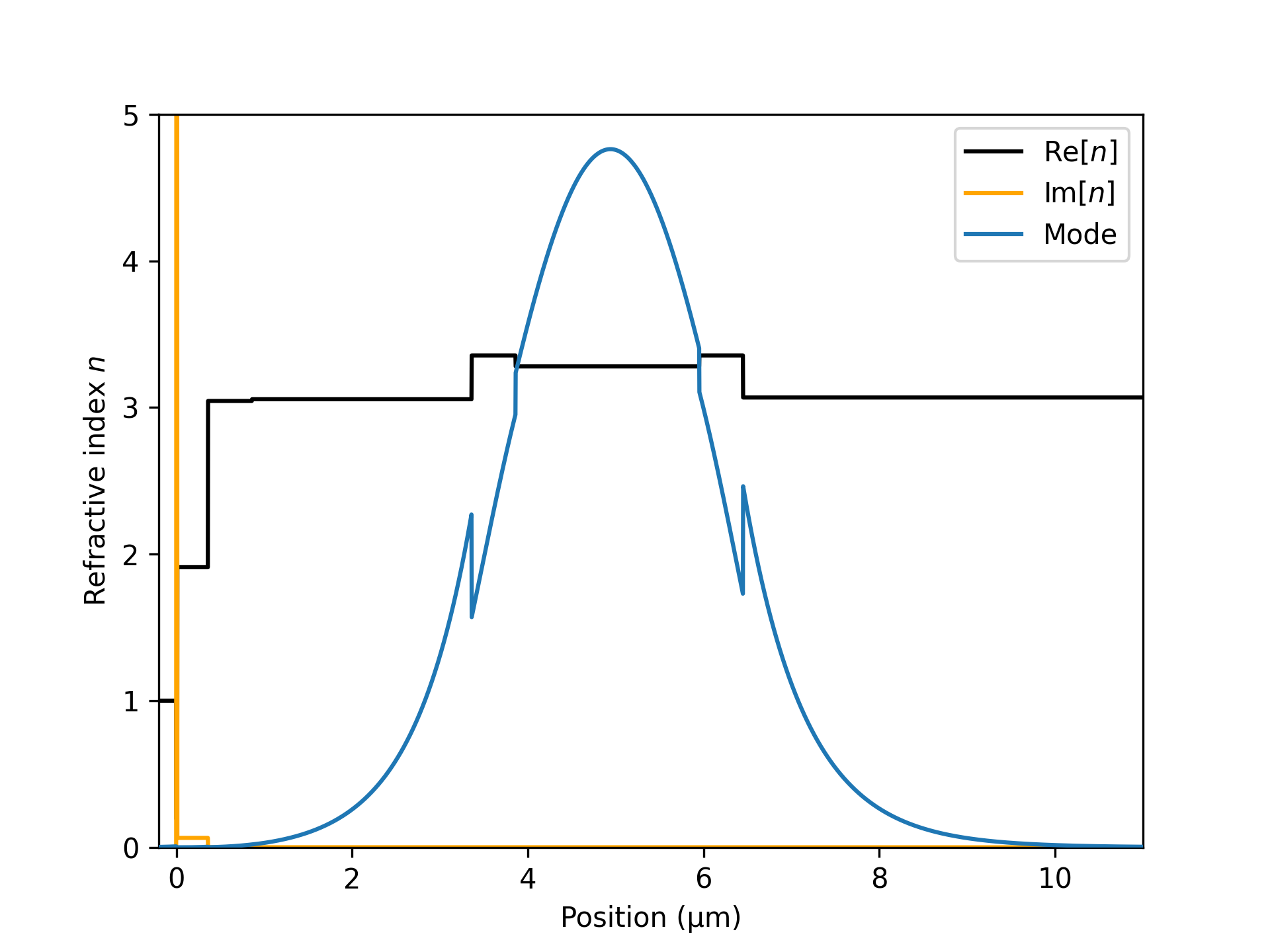
the guided mode, the confinement factor and plotting should be like:
xs = np.linspace(-1, sum(strata.Ls[1:]), 5000)
nx = strata.populateIndices(xs)
Ey, _, _ = strata.populateMode(beta, xs)
# confinement = strata.confinementy(beta, xs, Ey)

rIdxAxes = plt.gca()
modeAxes = rIdxAxes.twinx()
modeAxes.set_frame_on(False)
modeAxes.get_yaxis().set_visible(False)
rIdxAxes.set_xlabel('Position (μm)')
rIdxAxes.set_ylabel('Refractive index $n$')

lNReal = rIdxAxes.plot(xs, nx.real, 'k', label=r'$\mathrm{Re}[n]$')
lNImag = rIdxAxes.plot(xs, nx.imag, 'orange', label=r'$\mathrm{Im}[n]$')
lMode = modeAxes.plot(xs, np.abs(Ey)**2, color='C0', label=r'Mode')

lns = lNReal + lNImag + lMode
labs = [line.get_label() for line in lns]
plt.legend(lns, labs)
rIdxAxes.set_ylim(0, 5)
rIdxAxes.set_xlim(-0.2, 11)
modeAxes.set_ylim(bottom=0)

plt.show()
(Source code, png)

where matplotlib.axes.Axes.twinx() is used for plotting both the
refractive index and the mode.
Save the structure
Both the QC layers and the waveguide structure can be saved with
ErwinJr2.SaveLoad.EJSaveJSON().