OneDQuantum.OneDSchrodinger module

This module contains OneDSchrodinger functions. It is a Python interface of 1DSchrodinger.c

class ErwinJr2.OneDQuantum.OneDSchrodinger.Band(bandtype, *args, **kwargs)

Python interface for a Band

ErwinJr2.OneDQuantum.OneDSchrodinger.cBandFillPsi(step, EigenEs, V, band, xmin=0, xmax=None, Elower=None, Eupper=None, field=None)

Find wave functions using band mass. field, Elower and Eupper is used only for bound the energy range of the wave functions: outside the bound the wavefunction is promised to be zero.

Return type

ndarray

ErwinJr2.OneDQuantum.OneDSchrodinger.cBandSolve1D(step, Es, V, band, xmin=0, xmax=None)

Find eigen energies using band mass.

Return type

ndarray

ErwinJr2.OneDQuantum.OneDSchrodinger.cSimpleFillPsi(step, EigenEs, V, m, xmin=0, xmax=None)

Find wave functions. Assume mass as given.

Return type

ndarray

ErwinJr2.OneDQuantum.OneDSchrodinger.cSimpleSolve1D(step, Es, V, m, xmin=0, xmax=None)

Find eigen energies. Assume mass as given.

Return type

ndarray

Example

Here is an example for how to use OneDSchrodinger.py for 1D triangle well.

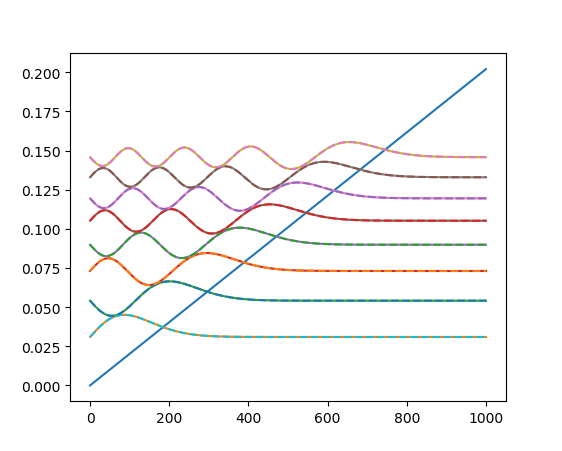
Output of SimpleSchrodinger.py

#!/usr/bin/env python3
# -*- coding:utf-8 -*-
from context import *
from OneDQuantum import *
from pylab import *
from scipy.constants import hbar, e, m_e, pi

ANG=1E-10


def square_well(x0=0, x1=100, x2=300, x3=400, Vmax=0.287):
    """
    Solve quantum for V = Vmax (x0<x<x1 or x2<x<x3), 0 (x1<x<x2)
    """
    x = np.linspace(x0, x3, 1000)
    step = x[1]-x[0]
    V = np.zeros(x.shape)
    V[(x < x1) | (x >= x2)] = Vmax
    mass = 0.067
    Es = np.linspace(0, 0.2, 100)
    EigenEs = cSimpleSolve1D(step, Es, V, mass)
    psis = cSimpleFillPsi(step, EigenEs, V, mass)
    print("Eigen Energy: ", EigenEs)
    plot(x, V)
    for n in range(0, EigenEs.size):
        plot(x, EigenEs[n] + psis[n, :]/np.max(psis[n, :])*0.01)
    return x, V, EigenEs, psis

def triangle_well(F, xmax=1E3):
    x = np.linspace(0, xmax, 5000)
    step = x[1]-x[0]
    V = F * (xmax - x)
    mass = 0.067
    Es = np.linspace(0, 0.15, 100)
    EigenEs = cSimpleSolve1D(step, Es, V, mass)
    psis = cSimpleFillPsi(step, EigenEs, V, mass)
    #  an = np.arange(0, 8) + 0.75
    #  EigenEs_th = (hbar**2/(2*m_e*mass*e*ANG**2)*(3*pi*F*an/2)**2)**(1/3)
    # Above is approximate Airy zeros result
    from scipy.special import airy, ai_zeros
    an = ai_zeros(8)[0]
    EigenEs_th = -(hbar**2*F**2/(2*m_e*mass*e*ANG**2))**(1/3)*an
    psis_th = np.array([
        airy((2*mass*m_e*e*ANG**2*F/hbar**2)**(1/3) * (x-E/F))[0]
        for E in EigenEs_th])
    psis_th /= (np.linalg.norm(psis_th, axis=1) * sqrt(step))[:, None]
    V = np.ascontiguousarray(V[::-1])
    psis = np.ascontiguousarray(psis[:, ::-1])
    print("Eigen Energy: ", EigenEs)
    print("Thoery: ", EigenEs_th)
    print("Diff: ", EigenEs - EigenEs_th)
    plot(x, V)
    scale = 0.15
    for n in range(0, EigenEs.size):
        plot(x, EigenEs[n] + psis[n, :]*scale)
    for n in range(0, EigenEs_th.size):
        plot(x, EigenEs_th[n] + psis_th[n, :]*scale, '--')
    return x, V, EigenEs, psis, EigenEs_th, psis_th


if __name__ == "__main__":
    x, V, EigenEs, psis = square_well()
    show()
    x, V, EigenEs, psis, EigenEs_th, psis_th = triangle_well(2.02e-4)
    show()